Sat 26 January 2008
Watersheds with lots of roads, buildings, parking lots, rock surfaces, compacted dirt, etc tend to prevent inflitration and cause rapid runoff in response to rainfall. This poses a number of challenges for managing stormwater and water quality. Not surprisingly, the percentage of hydrologically impervious surface in a given watershed is an important factor in many hydrologic models. Using standard aerial photography and GRASS, it's a relatively simple process to create an impervious surface map using supervised classification.
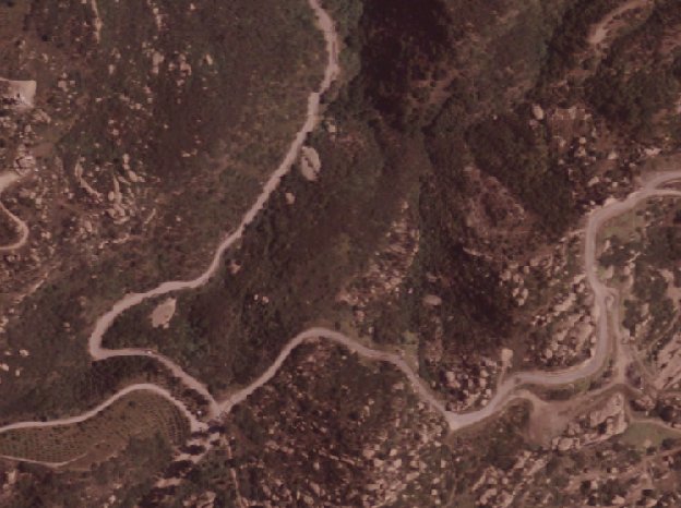
First find an aerial photo. I grabbed a NAIP image from CASIL but you might want to try using OpenAerialMap. The red, green and blue visible bands are usually sufficient for differentiating between impervious and pervious land use types... For distinguishing different types of vegetation you might want to use a multispectral imagery source with non-visible bands (ie near infrared) but this is usually lower resolution (eg. 30 meter pixels of Landsat) or much more expensive.
Next we jump into GRASS and import our image into a new location:
r.in.gdal -e input=naip.img output=naip location=impervious
Exit and log back into your new location. If you look at the imported rasters, you'll see three rasters, not one. Each band (R, G and B) gets imported separately.
GRASS 6.3.cvs (impervious):~/>  g.list rast
raster files available in mapset permanent:
naip.1 naip.2 naip.3
We need to indicate that these rasters form a logical group
i.group group=naip2 subgroup=naip2 input=naip.3@PERMANENT,naip.2@PERMANENT,naip.1@PERMANENT
i.target -c group=naip2
At any time you can list the rasters in a given group/subgroup to confirm.
i.group -l -g group=naip2 subgroup=naip2
Now the real heart of the process. We need to define "training areas" which are polygons around representative land use types. I used QGIS to load the aerial photo and create a new polygon layer with an integer attribute field called vegnum. I digitized a few rocks, paved areas, rooftops and dirt roads to represent the impervious areas to which I assigned vegnum=1. Then I selected some grasslands, forests, lakes and chaparral and assigned 2 as the vegnum. The next step is to load the polygon data into GRASS and rasterize it (in retrospect it would have just been easier to create the grass vector layer from scratch in QGIS to avoid the import step). Note that the vegnum field is specified as the raster value column.
v.in.ogr -o dsn=./training/train1_utm/train1_utm.shp output=train1 layer=train1_utm min_area=0.0001 type=boundary snap=-1
v.to.rast input=train1 output=train1 use=attr column=vegnum type=point,line,area layer=1 value=1 rows=4096
Next we use i.gensig to generate a spectral signature (the statistical profile; mean and covariance matrix of the input pixels) for the training areas.
i.gensig trainingmap=train1 group=naip2 subgroup=naip2 signaturefile=naip2_train1.sig
Now that we have a signature of impervious vs. non-impervious surfaces, we can use the maximum likelihood method to classify each pixel into the highest probability category.
i.maxlik group=naip2 subgroup=naip2 sigfile=naip2_train1.sig class=imperv
You might notice a slight speckled, noisy appearance due to things like shadows, reflections or imperfect training areas. Usually these small 1-pixel deviations are not interesting enough to keep so we can smooth out the image taking the mode (most comon) cell in a 3x3 window.
r.neighbors input=imperv output=imperv_mode method=mode size=3
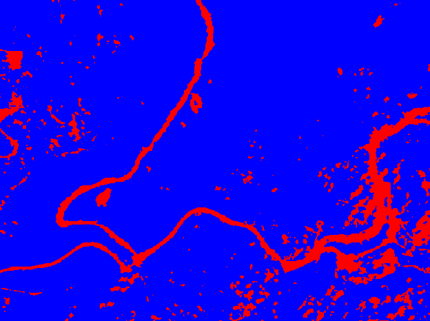
And here are the results... calculating imperviousness will most likely be an iterative process so be prepared to evaluate the output, tweak the training areas and rerun the process a few times. Once you're happy with the results, you can use zonal statistics with a tool like starspan to find the percent imperviousness of your watersheds or other regions.

