Sat 03 December 2005
NOAA Electronic Navigational Charts (ENC) contain (among many other things) depth soundings that can be processed into raster bathymetry grids. The ENC files are available as a huge torrent from geotorrent.org (http://geotorrent.org/details.php?id=58).
Download this torrent and check readme.txt to find the chart of interest:
Port Hueneme to Santa Barbara|5|2005-10-03|2005-10-03|US5CA65M
First check out the gdal documentation for s57 files at http://www.gdal.org/ogr/drv_s57.html.
Change to the US5CA65M directory and you'll see a .000 file (and maybe .001, .002 etc). Run ogrinfo on the .000 file and you'll see ~ 61 layers, one of which ("SOUNDG") represents the soundings. Let's start by examining the soundings layer:
ogrinfo -summary US5CA65M.000 SOUNDG
We see that there are 43 "features" but since the features are multipoints, there are actually thousands of soundings. The multipoints are 3D so If we convert to a shapefile with ogr2ogr's default settings we loose the 3rd dimension. To solve this, we need to append "25D" to the layer type. Furthermore, the multipoint geometry confuses some applications so we want to split it into a layer with simple 3D point geometries. Luckily there is a SPLIT_MULITPOINT option that must be specified as an environment variable:
export OGR_S57_OPTIONS="RETURN_PRIMITIVES=ON,RETURN_LINKAGES=ON,LNAM_REFS=ON,SPLIT_MULTIPOINT=ON,ADD_SOUNDG_DEPTH=ON"
ogr2ogr -nlt POINT25d test3.shp US5CA65M.000 SOUNDG
Now we get ~ 3000 3D points with the depth added as an attribute for good measure.
Now bring these into grass and create a raster:
v.in.ogr -zo dsn=test3.shp output=soundg layer=test3
v.info soundg
g.region vect=soundg nsres=0.001 ewres=0.001
v.surf.rst input=soundg elev=bathy layer=0
r.info bathy
since depths actually show up as positive elevations, we want to multiply the grid by -1
r.mapcalc sb_bathy=bathy*-1
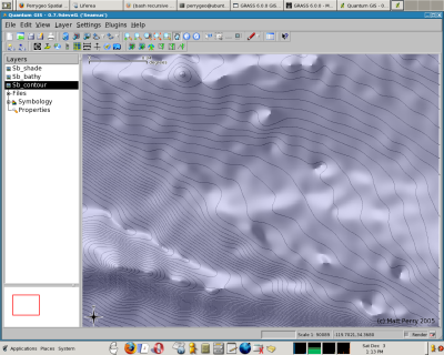
And of course we want to make some nice shaded relief and contour maps for viewing with QGIS:
r.shaded.relief map=sb_bathy shadedmap=sb_shade altitude=45 azimuth=315
r.contour input=sb_bathy output=sb_contour step=5
qgis &

From the screenshot, we see the pits and spikes from potential outliers so we might want to go back and adjust the tension and smoothing on the raster creation (the v.surf.rst command).