perrygeo

About | Articles | CV

Zonal Stats with PostGIS Rasters, part 2

Sat 28 November 2020

In my last post I compared two approaches for calculating zonal statistics:

A Python approach using the rasterstats library
A SQL approach using PostGIS rasters.

I came away happy that I could express zonal stats in SQL, but wasn't happy with the performance; an 87x slowdown compared to the equivalent Python code. When in doubt though, it's user error! I received some good suggestions from readers of this blog (Thanks Stefan Jäger and Pierre Racine!) who suggested some performance enhancements from tiling and spatial indexes.

Additionally, I wasn't happy with the setup of the last experiment; while PostGIS and Rasterio both interact with the underlying GDAL C API, in my experiment they were using GDAL libraries of different origins. And I'm skeptical that my synthetic vector data was representive of all workloads. A common case for zonal statistics is aggregating a raster by (non-overlapping) administrative boundaries. The nature of the datasets can have a significant impact; best to go with something more realistic.

Time for a reboot...

Reproducible containers

I used my docker-postgres image to easily recreate an environment where everything is built from source against the same shared libraries.

To run a postgresql server from a docker container (no messy install required) with local data volumes mounted in ./pgdata.

git clone https://github.com/perrygeo/docker-postgres.git
cd docker-postgres
./run-postgres.sh

This will download a pre-built image from Dockerhub so you can try it out without messing with your system. Then launches the Postgresql server process, with your local pgdata, mnt_data and log directories mounted as container volumes.

In order to run Python code from the same container, we can exec into it to get shell access:

docker exec -ti postgres-server /bin/bash

From here we can run our Python-based command line tools (Rasterio)

$ rio --version
1.1.8
$ rio --gdal-version
3.2.0

Connecting to the server with psql, I can use the built-in version commands to show what we're working with

SELECT version();

PostgreSQL 13.0 on x86_64-pc-linux-gnu, compiled by gcc (Debian 8.3.0-6) 8.3.0, 64-bit

SELECT postgis_full_version();

POSTGIS="3.1.0alpha3 b2221ee"
PGSQL="130"
GEOS="3.9.0dev-CAPI-1.14.0"
PROJ="7.2.0"
GDAL="GDAL 3.2.0, released 2020/10/26"
LIBXML="2.9.4"
LIBJSON="0.12.1"
LIBPROTOBUF="1.3.3"
WAGYU="0.5.0 (Internal)"
RASTER

Since the Rasterio library is running in the container, linked to exact same GDAL, GEOS and PROJ libraries as PostGIS, we can be assured of a more consistent environment.

Raster dataset

For our raster dataset, we'll use the historic climate data provided by the WorldClim project. For our experiment we'll use the historic average monthly temperature rasters.

wget http://biogeo.ucdavis.edu/data/worldclim/v2.1/base/wc2.1_2.5m_tavg.zip
unzip wc2.1_2.5m_tavg.zip

The result is a dozen monthly GeoTIFF files representing the historic average temperature for the month - we'll use wc2.1_2.5m_tavg_07.tif, the average July temperature. Each raster is a 4320 x 8640 grid with global coverage in WGS84 coordinates.

And use Rasterio to inspect the shape of the raster grid

rio info wc2.1_2.5m_tavg_07.tif | jq -c .shape

which prints to stdout, confirming the raster grid shape:

[4320,8640]

Vector data

For our vector dataset, we're using the Natural Earth Admin dataset with 241 multipolygons, one for each nation.

wget https://www.naturalearthdata.com/http//www.naturalearthdata.com/download/50m/cultural/ne_50m_admin_0_countries.zip
unzip ne_50m_admin_0_countries.zip

Check the number of features using Fiona

$ fio info  ne_50m_admin_0_countries.shp | jq .count
241

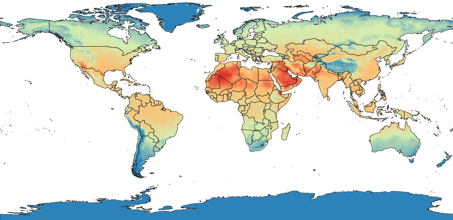
Overlaying the admin polygons on top of the stylized temperature raster and we get a good picture of the question we're trying to answer:

What is the historical average temperature of each country in the month of July?

Zonal Stats using `python-rasterstats`

from rasterstats import zonal_stats

stats = zonal_stats(
    vector="ne_50m_admin_0_countries.shp",
    raster="wc2.1_2.5m_tavg_07.tif",
    stats=["sum", "mean", "count", "std", "min", "max"]
)

The time to complete this script was 6.67 seconds (fastest of 3 runs).

Zonal Stats using `postgis_raster`

To test the performance of the database, we need to get the data in:

Load the raster data

In part 1, I imported my raster data using a rather naive raster2pgsql command. This time, we add a few more options to tune performance.

raster2pgsql -Y -d -t 256x256 -N '-3.4e+38' -I -C -M -n "path" \
    wc2.1_2.5m_tavg_07.tif tavg_07 | psql

The -t 256x256 is a key parameter. By cutting the raster into 256-pixel square tiles, the resulting raster table contains multiple rows, one per tile. A spatial index on the tiles, combined with rewriting the SQL to take advantage of the index and to aggregate across tiles, zonal stats can be made much more efficient inside PostgreSQL.

The -I indicates that a spatial index of the raster tiles should be built after import. The spatial index, along with a spatial query that can take advantage of it, can quickly select the subset of tiles that overlap your features of interest.

The other parameters to note:

-Y uses COPY for more efficient transfer.
-d deletes the table if it already exists (useful for testing but careful in production).
-N defines a nodata value directly at the CLI.
-n create a path column to store the filename.
-C applies constraints to ensure valid raster alignment, etc.
-M runs VACUUM ANALYZE on the table as a final step.

Load the vector data

Using a standard shp2pgsql with a -I to build and index.

shp2pgsql -g geometry -I -s 4326 ne_50m_admin_0_countries.shp countries | psql

Run the query

Now we have two tables loaded, countries and tavg_07, and can ask our question in SQL:

SELECT
    (ST_SummaryStatsAgg(ST_Clip(raster.rast, countries.geometry, true), 1, true)).*,
    countries.name AS name,
    countries.geometry AS geometry,
    count(1) as n_tiles
FROM
    tavg_07 as raster
INNER join countries on
    ST_INTERSECTS(countries.geometry, raster.rast)
GROUP BY
    name, geometry;

I added the GROUP BY to aggregate across tiles; otherwise we'd get multiple rows per country. And on the SELECT side, PostGIS provides a ST_SummaryStatsAgg function (the aggregate variant of the ST_SummaryStats) to sum across tiles.

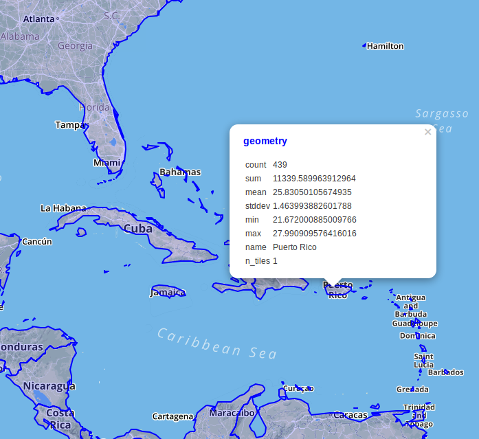
Here's the resulting map data rendered via DBeaver. The count is the number of raster pixels intersecting the feature, while the n_tiles is the number of raster tiles. The mean is probably what we're interested in; the avergage temperature.

Here's the bottom line on performance: PostGIS can perform this query in 6.1s. Marginally faster than the Python rasterstats version even. It could be that the latest improvements in the geospatial stack account for some of this effect but tiling clearly matters to performance.

Effect of tile size

The chosen value of -t determines how much data fits into each tile. There's an unavoidable inverse relationship between the size of a row and the number of rows/tiles. Not surprisingly we find a tradeoff between those two constraints.

tilesize	query (s)	raster2pgsql import (s)
64x64	5.9	58.7
256x256	6.6	15.8
1024x1024	8.5	7.3
untiled	49.2	5.2

Smaller tiles with a spatial index means more efficient queries, at the expernse of pre-chopping the raster into many tiles. Depending on the nature of your analysis, you'll want to adjust accordingly. The optimal tilesize is likely to depend on hardware, the tiling patterns of the orignal data and and the usage patterns you expect.

For this dataset, somewhere around 256x256 appears to be an optimal size. It would make a good default providing the benefits of tiling without as much import overhead as smaller tiles.

Surprisingly, the untiled version still performs ok relative to the python code. The query on an untiled raster is "only" 7.5x slower than the python code, not as bad as the 80x performance hit I found in part 1. While this factor seems highly dependent on the data at hand, the conclusion doesn't change - tiling maters.

Conclusion

Use raster2pgsql -t 256x256 -I to tile your PostGIS rasters. Combined with aggregate functions and spatial indexes, you get similar zonal stats query functionality and performance from PostGIS as you would with equivalent single-threaded Python/GDAL approaches.

There's still much to be explored regarding optimal tiling, parallel aggregates, out-of-band rasters, and the impact of source raster data file layout on performance. More to come in part 3...