perrygeo

About | Articles | CV

Zonal Stats with PostGIS Rasters

Mon 31 December 2018

Zonal statistics is a technique to summarize the values of a raster dataset overlapped by a set of vector geometries. The analysis can answer queries such as "Average elevation of each nation park" or "Maximum temperature by state".

My goal in this article is to demonstrate a PostGIS implementation of zonal stats and compare the results and runtime performance to a reference Python implementation.

Python with the rasterstats library using GeoTIFF and GeoJSON files.
SQL queries using PostGIS raster and vector tables.

The Dataset

For the raster data, let's use the ALOS Global Digital Surface Model (from the Japan Aerospace Exploration Agency ©JAXA). I picked a 1°x1° tile with 1 arcsecond resolution (roughly 30 meters) in GeoTIFF format.

Next, generate 100 random circular polygon features covering the extent of the raster. The following Python script shows how to do so with the Rasterio and Shapely libs.

#!/usr/bin/env python
import json
import random
import sys

import rasterio
from shapely.geometry import Point


def random_features_for_raster(path, steps=100):
    with rasterio.open(path) as src:
        x1, y1, x2, y2 = src.bounds

    xs = [random.uniform(x1, x2) for _ in range(steps)]
    ys = [random.uniform(y1, y2) for _ in range(steps)]
    for i, (x, y) in enumerate(zip(xs, ys)):
        buffdist = random.uniform(0.002, 0.04)
        shape = Point(x, y).buffer(buffdist)
        yield {
            "type": "Feature",
            "properties": {"name": str(i)},
            "geometry": shape.__geo_interface__,
        }


if __name__ == "__main__":
    for feat in random_features_for_raster(sys.argv[1]):
        print(json.dumps(feat))

Piping the features through fio collect gives us a valid GeoJSON collection with 100 polygon features.

python make-random-features.py N035W106_AVE_DSM.tif | fio collect > regions.geojson

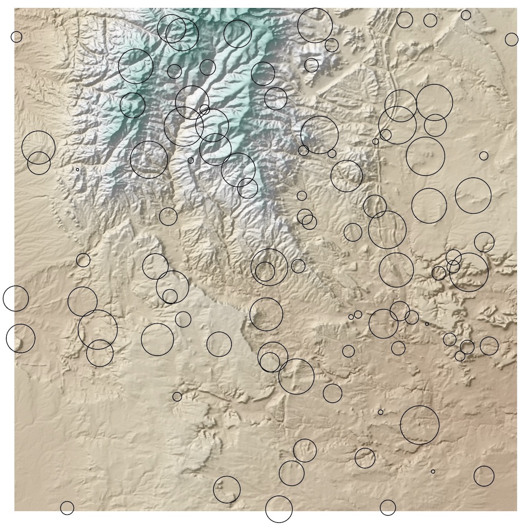
Visualizing the data in QGIS shows what we're working with. The goal is to find basic summary statistics for elevation in each of the regions:

Python with `rasterstats`

Using zonal_stats Python function allows you to express the processing at a high-level.

#!/usr/bin/env
import json
from rasterstats import zonal_stats

features = zonal_stats(
    "regions.geojson"
    "N035W106_AVE_DSM.tif"
    stats=["count", "sum", "mean", "std", "min", "max"],
    prefix="dem_",
    geojson_out=True)

with open("regions_with_elevation.geojson", "w") as dst:
    collection = {
        "type": "FeatureCollection",
        "features": list(features)}
    dst.write(json.dumps(collection))

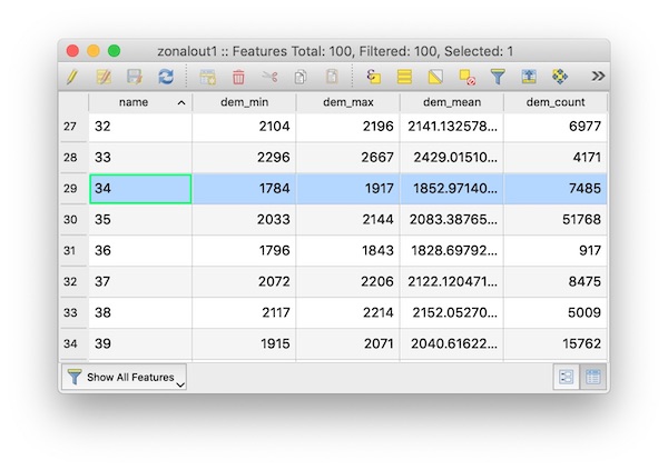
Running this script takes about 2.4 seconds and creates a new GeoJSON file regions_with_elevation.geojson with the following attributes, as viewed in QGIS

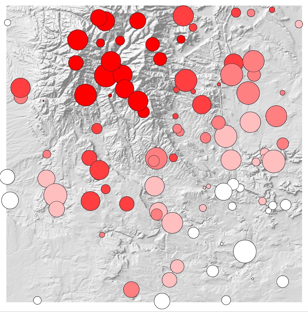
And the resulting features can be mapped, in this case using the dem_mean field to show the average elevation of each region:

Postgis

Instead of working with GeoTiff rasters and GeoJSON files, we can perform the same thing in PostGIS tables using SQL.

Loading the data

To create a raster table name dem from the GeoTIFF.

raster2pgsql N035W106_AVE_DSM.tif dem | psql <connection info>

For some rasters, it might be necessary to explictly set the nodata value.

UPDATE dem SET rast = ST_SetBandNoDataValue(rast, -32768);

To create a vector table named regions from the GeoJSON file. (See ogr2ogr docs for details on the connection info)

ogr2ogr -f PostgreSQL PG:"<connection info>" regions.geojson

Zonal Statistics in SQL

Now we can express our zonal stats analysis as a SQL statement.

SELECT
    -- provides: count | sum | mean | stddev | min | max
    (ST_SummaryStats(ST_Clip(dem.rast, regions.wkb_geometry, TRUE))).*,
    regions.name AS name,
    regions.wkb_geometry AS geometry
INTO
    regions_with_elevation
FROM
    dem, regions;

Let's break that down a bit

FROM dem, regions does a full product of the 100 regions X 1 raster row.
ST_Clip function clips each raster to the precise geometry of each feature.
ST_SummaryStats function summarizes each clipped raster and produces a count, sum, mean, standard deviation, min and max column.
INTO regions_with_elevation creates a new table with the results.

Conceptually, this approach is similar to the internal process used by rasterstats.

database=# SELECT name, min, max, mean, count from regions_with_elevation;

name | min  | max  |       mean       | count
-----+------+------+------------------+-------
...
32   | 2104 | 2196 | 2141.13257847212 |  6977
33   | 2296 | 2667 | 2429.01510429154 |  4171
34   | 1784 | 1917 | 1852.97140948564 |  7485
35   | 2033 | 2144 | 2083.38765260393 | 51768
36   | 1796 | 1843 | 1828.69792802617 |   917
37   | 2072 | 2206 |  2122.1204719764 |  8475
38   | 2117 | 2214 | 2152.05270513076 |  5009
39   | 1915 | 2071 | 2040.61622890496 | 15762
...

Compared to attribute table screenshot above, the results are identical for all columns. That isn't too surprising given that both approachs use GDAL's rasterization API under the hood.

Performance is a different story. The zonal stats query took 81.90 seconds, roughly 34x slower than the Python code for the equivalent result.

Thoughts

In terms of the expressiveness of the two approaches, I can see the appeal of both Python code and SQL queries. Of course this will be personal preference depending on your background and familiarity with the environments. The Python API hides the implementation details and is more flexible, with more statistics options and rasterization strategies. But the SQL approach covers the common use case in a declarative query; it exposes the implementation details yet remains very readable.

The performance impact is significant enough to be a deal breaker for PostGIS. I haven't delved into the issues too closely; There might some obvious ways to optimize this query but I haven't found anything as of writing this. PostGIS experts, please get in touch if you find any speedups that I could consider here!

Performance combined with the additional overhead of managing postgres instances and data imports tells me that running zonal stats in postgis will not be a great option unless you're already running PostgreSQL. If your application is already committed to postgres and you want to integrate zonal stats tightly into your data management strategy, it could be a viable approach. For example, you could create a TRIGGER or an asyncronous worker via LISTEN/NOTIFY to ensure run zonal statistics is run each time a new feature is inserted into your vector table.

For most other zonal stats use cases, using rasterstats against local files or in-memory Python data will be a faster with less data management overhead.